
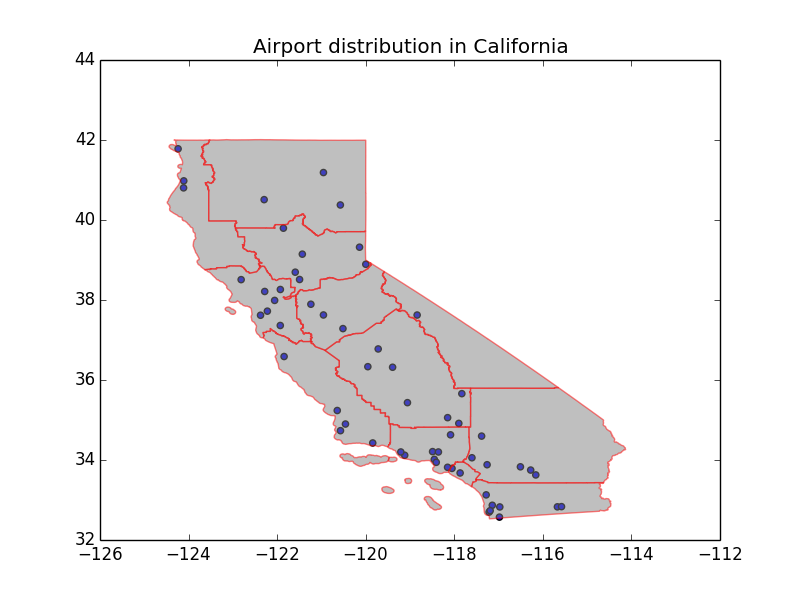
This python-based program examines the spatial pattern of airports in California by using K-function. The airport data at the National Atlas website includes more than 900 points in the country. This program uses airports in California as a subset to analyze the spatial pattern of these airports.
Visualization:
Import libraries and data. The data used by this program can be found here. Before handling the data, this program checks projection used in ’airprtx010g.shp’ and ‘District_201511.shp’ respectively. Since both shapefiles use the same projection, GCS_North_American_1983, there is no need to transform projection.
import csv
import numpy
from osgeo import ogr
from osgeo import osr
import matplotlib.pyplot as plt
import matplotlib.pyplot as plt
from point import *
from kdtree1 import *
from extent import *
from kfunction import *
from drawgeometry import *

# check projection
print '*****check projection*****'
print ''
driver = ogr.GetDriverByName("ESRI Shapefile")
shapefile = 'data/District_201511.shp'
vector = driver.Open(shapefile, 0)
layer = vector.GetLayer(0)
spatialRef = layer.GetSpatialRef()
print spatialRef
print ''
shapefile1 = 'data/airport/airprtx010g.shp'
vector1 = driver.Open(shapefile1, 0)
layer1 = vector.GetLayer(0)
spatialRef1 = layer1.GetSpatialRef()
print spatialRef1
print ''
print '*****done*****'

# import data from csv file
airports = []
lat =numpy.genfromtxt('data/airport.csv', usecols = (11), skiprows=1,delimiter=',')
lon =numpy.genfromtxt('data/airport.csv', usecols = (12), skiprows=1,delimiter=',')
states =numpy.genfromtxt('data/airport.csv', usecols = (7), skiprows=1,delimiter=',')
for i in range(len(states)):
    if states[i] == 6:    # 6 is the index number of CA in the shapefile
        airports.append((lon[i],lat[i]))
The program extracts the data from the 7th(index of states), 11th(latitude), and 12th(longitude) columns. Selected data will be store in a list named ‘airports’. Then, all data representing airports in California will be filtered. This part could be replaced by other index numbers if you want to look into airports in other states. Point pattern analysis is based on a radius stepping on 10 intervals divided by 2/3 of the width the area.
# point pattern analysis
points = [Point(d[0],d[1]) for d in airports]
extent = layer.GetExtent()
area = Extent(xmin=extent[0], xmax=extent[1], ymin=extent[2], ymax=extent[3])
n = len(points)
density = n/area.area()
t = kdtree2(points)
d = min([area.xmax-area.xmin, area.ymax-area.ymin])*2/3/10
ds = [ d*(i+1) for i in range(10)]
lds = [0 for d in ds]
for i, d in enumerate(ds):
    for p in points:
        ld = kfunc(t, p, d, density)[1]
        lds[i] += ld
lds = [ld/n for ld in lds]

# plot kfunction
plt.plot(ds, lds, color='grey', label='Data')
plt.xlabel('Radius ($d$)')
plt.ylabel('$L(d)$')
plt.title('K Function ($\lambda$ = {0:5.2f})'.format(density))
plt.plot([0, plt.xlim()[1]], [0, plt.xlim()[1]], color='r', label='Random')
plt.legend(loc='upper left')
plt.show()

# plot airport distribution
draw_layer(layer, plt)
vector.Destroy()
plt.title('Airport distribution in California')
airports_lat = [i[0] for i in airports]
airports_lon = [i[1] for i in airports]
plt.scatter(airports_lat, airports_lon, c='blue')
plt.show()
-
Test Results:
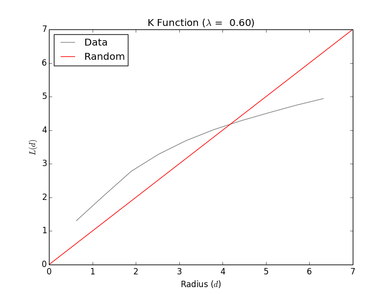 The observed spatial pattern curve is above the expected random spatial pattern line at low radius and L(d), which indicates statistically significant clustering at smaller distance. However, at high radius and L(d), the observed spatial pattern curve is below the expected random spatial pattern line, which indicates statistically significant dispersion at larger distances. Overall, 2/3 part of observed segment is above the expected random spatial pattern.
 -
Interpreting K Function Results: As referred from the test result above, the spatial pattern of airports in California is more clustered than chance would have it.
-
Limitation: According this program, the test area was built based on the envelope of all airports, which significantly increased the actual area of California.